Grouping Multiple Ranges in Excel

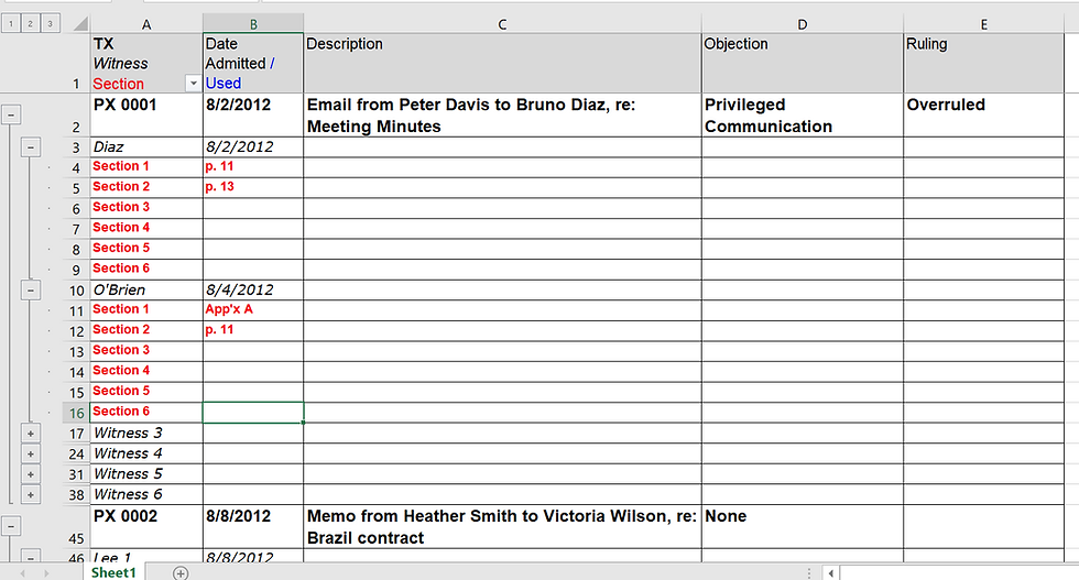
Tonight's tip will show how to group multiple ranges of rows on a worksheet using Excel's Auto Outline tool. In this particular example I'm setting a spreadsheet to track trial exhibit admissions. The trial exhibits will be on the first level. The witness each exhibit is used for will be on the second tier, and the third group will be used to keep track of which page, section, appendix, or other division of a trial exhibit is discussed during the testimony of a witness.

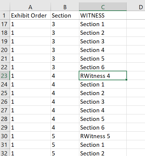
The key is to set up a worksheet with numbers listed on the bottom level, and then SUM formulas referring to these numbers on the top and middle levels. Begin by setting up a spreadsheet as shown below, with six sections listed for each witness, and six witnesses for each exhibit. (Obviously this can be varied depending on how often you think an exhibit will be used, and how many of its parts will be referenced.) I'm assuming that someone setting up this spreadsheet will have a basic familiarity with Excel and have no trouble setting up the entries in each column using IF . . . THEN formulas, and other common techniques. I will try to find time another night to demonstrate how this is done.

Column A should have one number repeated 42 times for each number. Six sections repeated six times, for six witnesses. If you have 10 trial exhibits there will be 420 entries in the first column. In Column B, each witness will be counted, continuing sequentially when a new exhibit is reached. For 10 exhibits, the count will be 60 at the end of 420 entries.

At the bottom of the worksheet add the list of exhibits in column C, with 1 repeated in column B for each exhibit, and in column A a number to count each exhibit.

Put an R in front of each occurrence of 'Witness' so it will sort in order after PX or DX numbers and before the Section references.

Sort by column A, column B. and then column C. This will put an exhibit number before each set of six witnesses, and each set of six sections between witnesses. Next, filter in column C for 'Section' and then add a '1' in column D for each displayed cell. Then filter in column C for 'Witness' and in the displayed cells in column D enter a sum folder adding up the values in the section cells. So as shown here, add D4 through D9, the cells between the filtered cell D3 and D10, and pull the formula down using CTRL + D.

Next in column D, add in a SUM formula referring to each of the cells in column D for which there's an entry on the same row in column C in which a witness is referenced, every seventh cell.

Filter in column C for 'PX' and pull this formula down. Now we have a mathematical structure Excel can analyze, with each cell on the second level referencing all of the numbers on the third 'section' level, and each cell on the top 'exhibit' level using a formula to reference all of the SUM results on the second level. Leaving the formulas active in column D, remove the first two columns and correct the spelling of 'RWitness'. Select only the cells in the data range (not the full columns or rows) and then expand the Outline section on the Data ribbon. Uncheck 'Summary rows below detail' and 'Summary columns to right of detail', and check 'Automatic styles'. Click the 'Create' button.

You will now have a collapsible exhibit list which can be expanded to enter multiple witness names, and page references.

If the 'Generate' column with the formulas is removed, the worksheet will retain the group levels. You can add more columns as necessary to track exhibit admissions.

It occurred to me today that this format would be particularly useful to track exhibit admissions. It will avoid the need to put multiple witness names on separate lines inside a cell, or extend the worksheet many columns to the right to have a separate column for each witness name. But naturally this tip can be applied to a wide range of circumstances when dealing with all kinds of data.