Pull Data by Referencing Column Headings on Multiple Worksheets

This Tip of the Night shows how to search for column headings on multiple worksheets of an Excel spreadsheet, when the worksheets don't necessarily have columns with common headings in the same order. The worksheet to which the results of the formulas will be pulled, contains a reference number in one column, and a second column listing the name of the worksheet on which the reference number appears. A formula is used which will refer to those two columns and the column headings.

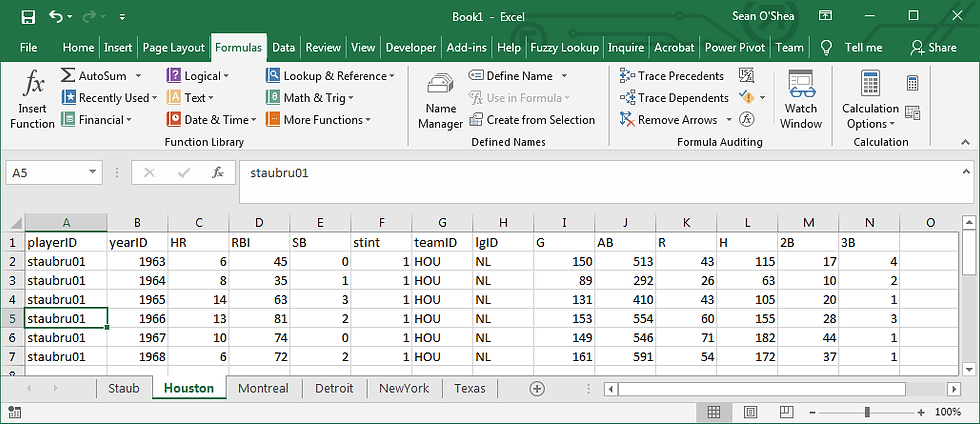
In this example, we want to add in the batting statistics for Rusty Staub on the first worksheet, when this data is listed on separate worksheets - each named with a different city he played in. The reference or control number is the year of a baseball season. Each worksheet with the data to be pulled has his stats in a different order:

Under the first column for which we want to pull data we enter this formula:

=HLOOKUP(D$1,INDIRECT("'"&$B2&"'!A:AZ"),MATCH($A2,INDIRECT("'"&$B2&"'!B:B"),0),FALSE)

This is a simple HLOOKUP formula which includes other formulas. Here's a breakdown

1. =HLOOKUP(D$1 - finds the value in the heading. An absolute reference is entered to the first row so when the formula is pulled down for subsequent years, it continues to enter the heading for each statistic.

2. INDIRECT("'"&$B2&"'!A:AZ") - this formula is used to enter worksheet reference in the HLOOKUP formula

3. MATCH($A2, - search for the control number - the season year in this example - so HLOOKUP knows which row to pull data from after it finds the heading.

4. INDIRECT("'"&$B2&"'!B:B"),0),FALSE) - the reference to the worksheet is entered again, to search on each worksheet for the control number. It is necessary for the reference number (the season year in this example) to appear in the same column on each worksheet.