


Table Specifiers
Get to know how to use specifiers in Excel tables. These can ease the entry of cell references in formulas.
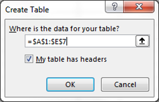
Begin by putting data on a worksheet in table. Press, CTRL + T, and then select a range of data, indicating if you already have column headers.

When you start to enter a formula, Excel will prompt you to select existing tables. You can specify the name of a column heading in brackets. E.g., =MAX(Table5[Sales Amount])


With the specifier #Data in the brackets, Excel will review all of the data in table except for the column headings. E.g., =MAX(Table5[#Data])


Using the @ symbol in brackets after the formula will find the value for a column in the row the formula is entered in. E.g., =Table5[@Sales Amount] finds the amount in column C in row 4 in the below example.

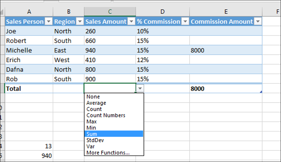
On the Table Tools Design tab check off 'Total Row', to add a new row to the bottom of a table which can be used to add in calculations for the figures listed in the above cells. Drop down menus will appear from which you can select formulas to calculate the sum, maximum, minimum, average and other values.
When the specifier #Totals is entered in a formula it will find the amount given in the total row in a particular column. E.g., =Table5[[#Totals],[Sales Amount]]
